Examples

This chapter details several models that were developed as I was writing this node library. Many of them are in note form but may be useful to the reader.

Constrained Gear System

This gear system was discovered while exploring planetary gears. It is constrained in the sense that the driven gears eventually engage the driving gear and to do that they must meet a certain criteria. The illustration below is a working system with \(Z_1\) and \(Z_3\) having 16 teeth, and the \(Z_2\) gears having 24. The angles, \(\theta_1\) and \(\theta_2\), are both equal to \(45^\circ\).

A constrained gear system, annotated.

Letting \(Z_1, Z_2\), and \(Z_3\) represent the number of teeth in the gears above, the constraint is this:

\begin{eqnarray} {Z_1\theta_1\over{180}}+{{Z_2(180+\theta_1+\theta_2)}\over{180}}+{{Z_3\theta_2}\over{180}}\in\mathbb{Z} \end{eqnarray}

That is, the left side of the equation must yield a whole integer. This seemingly odd requirement makes sense if you imagine a looping belt engaging in the teeth around \(Z_1\), then to the right side of \(Z_2\), around \(Z_3\), then the inside of \(Z_2\). If the belt is to be constantly engaged, its length must represent a whole number of teeth.

Universal Joint

Having never really thought much about universal joints I was surprised to learn that the rotational velocity is not even from one shaft to another when the shafts are not co-planar. If you were to animate this without the Blender physics engine, you will need to derive these uneven rotational angles. There are a number of approaches to this and, when I finish with this, I will probably discover that I’ve chosen the hardest way. Let’s start with the nice diagram provided by the wiki article:

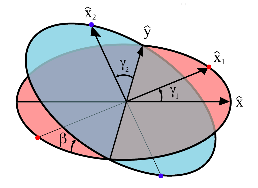
Variables for the universal joint

Expanding a little on the details provided by the wiki, I’ve made some derivations here that are more relevant to an implementation in Blender geometry nodes:

\(\hat{X_1}\) is confined to the “red plane” and is related to gamma_1 by:

\begin{eqnarray} \hat{X_1} = [ \cos\gamma_1, \sin\gamma_1, 0 ] \end{eqnarray}

This relates directly to the red plane lying flat on the XY plane in Blender and \(\gamma_1\) being a positive rotation about the Z axis.

Looking at the next paragraph in the wiki article regarding \(\hat{X_2}\), think of the vector \(\hat{X}=[1,0,0]\) rotating \(90^\circ\) (\(\pi\over{2}\)) on the X-axis, then \(\beta\) on the Y-axis, then rotated \(\gamma_2\) on the Z-axis. Trying not to repeat the wiki article completely, this results in an equation for motion as:

\begin{eqnarray} \tan\gamma_1 = \cos\beta\tan\gamma_2 \end{eqnarray}

Think of \(\gamma_1\) as the driving rotation which will result in rotating the other shaft \(\gamma_2\) degress on its blue plane when tilted at \(\beta\) degrees. Since Blender nodes don’t provide a \(\sec\) node because it is redundant to \(1\over{\cos}\), we can flesh out the derivation of \(\gamma_2\) as:

\begin{eqnarray} \tan\gamma_2 & = & \tan\gamma_1\over{\cos\beta} \\ \gamma_2 & = & \tan^{-1}({\tan\gamma_1\over{\cos\beta}}) \\ & = & \tan^{-1}({{\sin\gamma_1\over{\cos\gamma_1}}\over{\cos\beta}}) \\ & = & \tan^{-1}({\sin\gamma_1\over{\cos\gamma_1\cos\beta}}) \\ & = & atan2(\sin\gamma_1,\cos\gamma_1\cos\beta) \\ \end{eqnarray}

This gives us a Blender math node we can use.

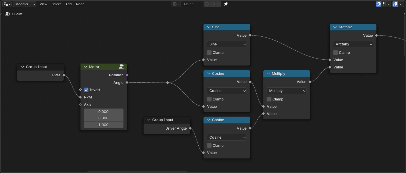
Calculating \(\gamma_2\) in geometry nodes.